Effect of sample timing (R example)
sample_timing.RmdIn this vignette, we will demonstrate the following tools:
- Using {mipdtrial} to simulate a trial, with the trial design specified using R code.
- We will have two trial “arms”, varying only by the therapeutic drug
monitoring strategy used. The two arms will be defined by two different
calls to
create_sampling_design()
Motivation
A hospital currently collects two samples for adjusting vancomycin doses: one at 1-hr post-dose and another at 9 hours post-dose. They want to compare the impact on target attainment (an area under the curve (AUC) of 400-600 mg*h/L) if they were to switch to collecting a single sample at 5 hours post-dose.
Here is how we could answer that problem using simulation!
library(mipdtrial)
library(dplyr)   # for easier data manipulation
library(tidyr)
library(ggplot2) # for plotting our results
if(!requireNamespace("pkvancothomson", quietly = TRUE)) {
  PKPDsim::install_default_literature_model("pk_vanco_thomson")
  loadNamespace("pkvancothomson")
}
1. Define trial design
This simulated trial will have two arms:
- Two samples, collected 1 and 9 hours after a dose
- One sample, collected 5 hours after a dose
In each case, we will collect the samples in the fourth dosing interval, and for simplicity, we will assume all patients are receiving vancomycin twice daily, infused over 2 hours.
tdm_design1 <- create_sampling_design(
  offset = c(1, 9),
  at = c(4, 4),
  anchor = "dose"
)
tdm_design2 <- create_sampling_design(
  offset = 5,
  at = 4,
  anchor = "dose"
)
We will adjust the fifth dose based on these levels, aiming for a daily AUC of 400-600 mg*h/L by day 6. We will use the Thomson (2009) model for simulating patient pharmacokinetics.
update_design <- create_regimen_update_design(
  at = 5,
  anchor = "dose",
  dose_optimization_method = map_adjust_dose,
  settings = list(
    dose_resolution = 50
  )
)
target_design <- create_target_design(
  targettype = "auc24",
  targetmin = 400,
  targetmax = 600,
  at = 6,
  anchor = "day"
)
model_design <- create_model_design(lib = "pkvancothomson")
Our initial dosing strategy will be based on population PK parameters, with dose size calculated to reach the specified target for a dosing interval of 12 hours.
initial_method <- create_initial_regimen_design(
  method = model_based_starting_dose,
  regimen = list(
    interval = 12,
    type = "infusion",
    t_inf = 1
  ),
  settings = list(
    auc_comp = 3,
    dose_resolution = 50,
    dose_grid = c(250, 5000, 250)
  )
)
Now we can combine all these design choices together:
design1 <- create_trial_design(
  sampling_design = tdm_design1, # arm 1
  target_design = target_design,
  regimen_update_design = update_design,
  initial_regimen_design = initial_method,
  sim_design = model_design, est_design = model_design
)

design2 <- create_trial_design(
  sampling_design = tdm_design2, # arm 2
  target_design = target_design,
  regimen_update_design = update_design,
  initial_regimen_design = initial_method,
  sim_design = model_design, est_design = model_design
)
2. Create a set of digital patient covariates
For this example, we will randomly generate a set of weights and creatinine clearances (CRCLs) for our synthetic data set.
set.seed(15)
dat <- data.frame(
  ID = 1:30,
  weight = rnorm(30, 90, 25),               # kg, normally distributed
  crcl = exp(rnorm(30, log(6), log(1.6)))   # L/hr, log-normally distributed
)
We will use the Thomson (2009) model, which accepts additional clearance from hemodialysis as a covariate. Let’s set that to zero in our data set.
Other models might require fat-free mass or other calculated covariates. This would be a good time to do that sort of processing on your data set!
dat$CL_HEMO <- 0Here are the first few rows of our data set:
head(dat)
#>   ID    weight      crcl CL_HEMO
#> 1  1  96.47057  4.827349       0
#> 2  2 135.77802  6.013269       0
#> 3  3  81.50954 11.863322       0
#> 4  4 112.42995  8.546496       0
#> 5  5 102.20041  9.448520       0
#> 6  6  58.61535  7.477850       0
We also need to link the covariates in our data set to the covariates expected in the model:
-
To check which covariates are required for your model use
PKPDsim::get_model_covariates():PKPDsim::get_model_covariates(model_design$model) #> [1] "WT" "CRCL" "CL_HEMO" -
To check which covariates are in your data set use
colnames():colnames(dat) #> [1] "ID" "weight" "crcl" "CL_HEMO"
cov_map <- c(
  WT = "weight",
  CRCL = "crcl",
  CL_HEMO = "CL_HEMO"
)
3. Simulate a trial!
Patients will get a model-based dose (using population PK parameters), and then this dose will be adjusted based on the MAP Bayesian fit made using the collected samples.
Individual PK parameters will be randomly generated based on the interindividual variability described in the model, and residual variability will be added to each sample collected using the error model described in the model.
res1 <- run_trial(
  data = dat,
  design = design1,
  cov_mapping = cov_map,
  progress = FALSE,
  seed = 15,
  n_ids = 3
)
#> ℹ Starting simulations in 1 threads
#> ℹ Post-processing results
res1$dose_updates
#>    t dose_update t_adjust dose_before_update interval_before_update
#> 1  0           5       48               1250                     12
#> 2 48          NA       NA               1500                     NA
#> 3  0           5       48               1550                     12
#> 4 48          NA       NA               1750                     NA
#> 5  0           5       48               3650                     12
#> 6 48          NA       NA               2950                     NA
#>   auc_before_update trough_before_update id
#> 1          461.2144            11.655690  1
#> 2          545.4241            13.727542  1
#> 3          624.9041            18.732721  2
#> 4          694.2896            20.758610  2
#> 5          546.3356             6.306444  3
#> 6          444.6457             5.190568  3

res2 <- run_trial(
  data = dat,
  design = design2,
  cov_mapping = cov_map,
  progress = FALSE,
  seed = 15
)
#> ℹ Starting simulations in 1 threads
#> ℹ Post-processing results
We can look at final exposure estimates for each arm:
final_exp1 <- res1$final_exposure %>%
  mutate(arm = "peak-trough")
final_exp2 <- res2$final_exposure %>%
  mutate(arm = "mid-interval")
results <- bind_rows(final_exp1, final_exp2)
head(results)
#>   id auc_true  auc_est tta target_index          arm
#> 1  1 545.4241 493.6145  25            1  peak-trough
#> 2  2 694.2896 497.3185  25            1  peak-trough
#> 3  3 444.6457 499.0814 121            1  peak-trough
#> 4  1 494.8983 507.5171  25            1 mid-interval
#> 5  2 746.3287 506.0676  25            1 mid-interval
#> 6  3 437.3822 502.4975 121            1 mid-interval
4. Analyze results
We are interested in AUC target attainment. How did target attainment compare between the two arms of the trial?
target_attainment <- results %>%
  mutate(ontarget = ifelse(auc_true >= 400 & auc_true <= 600, 1, 0)) %>%
  group_by(arm) %>%
  summarize(prop_on_target = 100 * mean(ontarget))
target_attainment %>%
  ggplot() +
    aes(x = arm, y = prop_on_target) +
    geom_bar(stat = "identity") +
    theme_minimal() +
    theme(
      panel.grid.major.x = element_blank()
    ) +
    labs(
      x = "Sampling strategy",
      y = "Percent on target (%)"
    )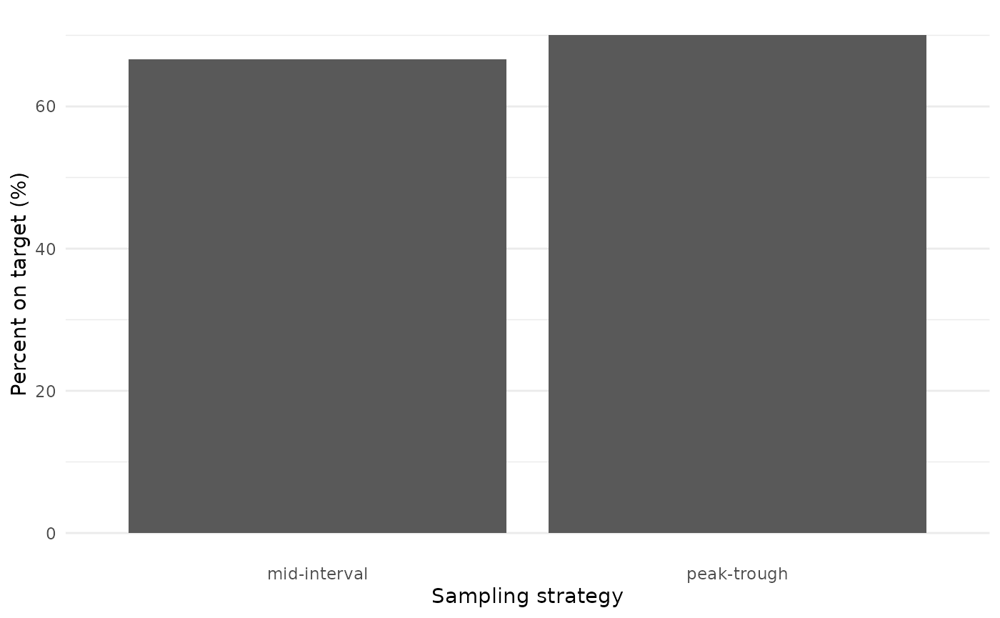
Target attainment was high and varied little between the two arms, providing evidence to support the move from collecting two samples to collecting a single sample per dosing interval.
Because we are simulating each sampling strategy in each patient, we can also look at how each patient responded to each sampling strategy.
results %>%
  select(id, auc_true, arm) %>%
  pivot_wider(names_from = arm, values_from = auc_true) %>%
  ggplot() +
    aes(x = `peak-trough`, y = `mid-interval`) +
    geom_rect(
      aes(xmin = 400, xmax = 600, ymin = -Inf, ymax = Inf),
      fill = "grey70",
      alpha = 0.05
    ) +
    geom_rect(
      aes(ymin = 400, ymax = 600, xmin = -Inf, xmax = Inf),
      fill = "grey70",
      alpha = 0.05
    ) +
    geom_point() +
    theme_minimal()
#> Warning: Removed 27 rows containing missing values or values outside the scale range
#> (`geom_point()`).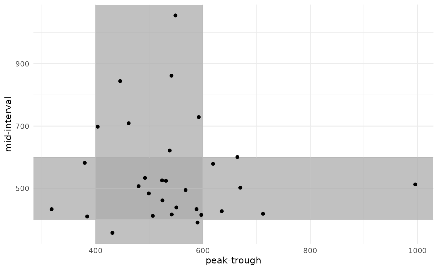
There is a strong correlation in final AUC between the two sampling strategies. Some patients were under-exposed or over-exposed in both strategies, while others were on-target in one strategy but not in the other.