Neutropenia (PKPD) • PKPDposterior

This examples shows how to implement the Friberg neutropenia model. What is implemented here is a generic version of it, i.e. not for a specific drug. We will sample from the posterior for the individual patients using TDM data and neutrophil count data.

We will first create the Stan model and sample from the posterior.

First, we define the model and parameters. Note that in this exmaple we specify ruv as a list that contains separate residual errors for pk- and pd-labeled observations.

parameters <- list(CL = 5, V = 50,
                   SLOPE = 0.1, MTT = 100, 
                   CIRC0 = 5, GAMMA = 0.2)
iiv <- list(
  CL = 0.2, V = 0.5, 
  SLOPE = 1.0, MTT = 0.2, 
  CIRC0 = 0.5, GAMMA = 0.2
)
ruv <- list(
  pk = list(add = 0.2),
  pd = list(add = 0.3)
)
parameter_definitions <- list(
  "CL" = "CL",
  "Q" = 0,
  "V" = "V",
  "V2" = 1,
  "KA" = 0,
  "MTT" = "MTT",
  "CIRC0" = "CIRC0",
  "GAMMA" = "GAMMA",
  "ALPHA" = "SLOPE"
)
ode <- "
  real ka  = 0;
  real k10 = CL / V;
  real k12 = 0;
  real k21 = 0;
  real ktr = 4 / MTT;
  
  real conc;
  real EDrug;
  real transit1;
  real transit2;
  real transit3;
  real circ;
  real prol;
  
  dAdt[1] = -KA * A[1];
  dAdt[2] =  KA * A[1] - (k10 + k12) * A[2] + k21 * A[3];
  dAdt[3] = k12 * A[2] - k21 * A[3];
  conc = A[2] / V;
  
  EDrug = ALPHA * conc; // slope model, not Emax
  prol = A[4] + CIRC0;
  transit1 = A[5] + CIRC0;
  transit2 = A[6] + CIRC0;
  transit3 = A[7] + CIRC0;
  circ = fmax(machine_precision(), A[8] + CIRC0); // Device for implementing a modeled 
  
  // initial condition
  dAdt[4] = ktr * prol * ((1 - EDrug) * ((CIRC0 / circ)^GAMMA) - 1);
  dAdt[5] = ktr * (prol - transit1);
  dAdt[6] = ktr * (transit1 - transit2);
  dAdt[7] = ktr * (transit2 - transit3);
  dAdt[8] = ktr * (transit3 - circ);
"

model <- new_stan_model(
  parameters = parameters,
  parameter_definitions = parameter_definitions,
  ode = ode,
  covariate_definitions = NULL,
  solver = 'pmx_solve_rk45',
  obs_types = c("pk", "pd"),
  custom_ipred = list(
    "pk" = "A[2, ] ./ V;",
    "pd" = "A[8, ] + theta[7];"
  ),
  verbose = T
)
model_file <- write_stan_model(model)

and compile the model:

mod <- load_model(
  model_file
)

Define the input data and prepare for use in Stan. Note that in the definition of tdm_data we use the type argument to distinguish between PK and PD observations.

regimen <- new_regimen(
  amt = 1500, 
  n = 3, 
  times = c(0, 24, 48), 
  type = 'infusion',
  cmt = 2,
  t_inf = 2
)
covariates <- NULL
tdm_data <- data.frame(
  t = c(2.5, 11.5), 
  dv = c(40, 14),
  type = "pk"
)
pd_data <- data.frame(
  t = c(3, 6, 9, 12) * 24, 
  dv = c(5, 1.5, .8, 2),
  type = "pd"
)
comb_data <- rbind(
  tdm_data, 
  pd_data
)

data <- new_stan_data(
  regimen,
  covariates = covariates, 
  data = comb_data,
  parameters = parameters,
  iiv = iiv,
  ltbs = list(pk = TRUE, pd = TRUE),
  ruv = ruv,
  dose_cmt = 2
)

Then, we can sample from the posterior using:

post <- get_mcmc_posterior(
  mod = mod,
  data = data
)

## Running MCMC with 1 chain...
## 
## Chain 1 Iteration:   1 / 1000 [  0%]  (Warmup) 
## Chain 1 Iteration:  50 / 1000 [  5%]  (Warmup) 
## Chain 1 Iteration: 100 / 1000 [ 10%]  (Warmup) 
## Chain 1 Iteration: 150 / 1000 [ 15%]  (Warmup) 
## Chain 1 Iteration: 200 / 1000 [ 20%]  (Warmup) 
## Chain 1 Iteration: 250 / 1000 [ 25%]  (Warmup) 
## Chain 1 Iteration: 300 / 1000 [ 30%]  (Warmup) 
## Chain 1 Iteration: 350 / 1000 [ 35%]  (Warmup) 
## Chain 1 Iteration: 400 / 1000 [ 40%]  (Warmup) 
## Chain 1 Iteration: 450 / 1000 [ 45%]  (Warmup) 
## Chain 1 Iteration: 500 / 1000 [ 50%]  (Warmup) 
## Chain 1 Iteration: 501 / 1000 [ 50%]  (Sampling) 
## Chain 1 Iteration: 550 / 1000 [ 55%]  (Sampling) 
## Chain 1 Iteration: 600 / 1000 [ 60%]  (Sampling) 
## Chain 1 Iteration: 650 / 1000 [ 65%]  (Sampling) 
## Chain 1 Iteration: 700 / 1000 [ 70%]  (Sampling) 
## Chain 1 Iteration: 750 / 1000 [ 75%]  (Sampling) 
## Chain 1 Iteration: 800 / 1000 [ 80%]  (Sampling) 
## Chain 1 Iteration: 850 / 1000 [ 85%]  (Sampling) 
## Chain 1 Iteration: 900 / 1000 [ 90%]  (Sampling) 
## Chain 1 Iteration: 950 / 1000 [ 95%]  (Sampling) 
## Chain 1 Iteration: 1000 / 1000 [100%]  (Sampling) 
## Chain 1 finished in 57.2 seconds.

Summary info about the posterior:

post

## Parameters:
##       posterior_mode   mean median    sd     q5     q95  rhat
## CL             4.069  4.220  4.201 0.539  3.355   5.132 1.006
## V             34.584 36.997 36.002 7.330 26.283  50.079 1.001
## SLOPE          0.060  0.059  0.058 0.016  0.035   0.086 0.998
## MTT           94.742 95.011 94.716 8.627 81.397 109.523 0.999
## CIRC0          5.014  5.686  5.464 1.440  3.742   8.090 1.003
## GAMMA          0.186  0.204  0.197 0.041  0.148   0.279 1.004
## 
## Observed data, posterior:
##   type  time   dv       mean         loc   pct       pct5     pct95
## 1   pk   2.5 40.0 35.1969640 -----|---o- 0.808 26.0733850 45.252310
## 2   pk  11.5 14.0 12.1645054 -----|---o- 0.838  9.3491765 15.305140
## 3   pd  72.0  5.0  4.5255091 -----|--o-- 0.708  3.1641995  6.190220
## 4   pd 144.0  1.5  1.7014853 --o--|----- 0.278  1.1376500  2.271029
## 5   pd 216.0  0.8  0.8655025 ---o-|----- 0.436  0.5374418  1.301487
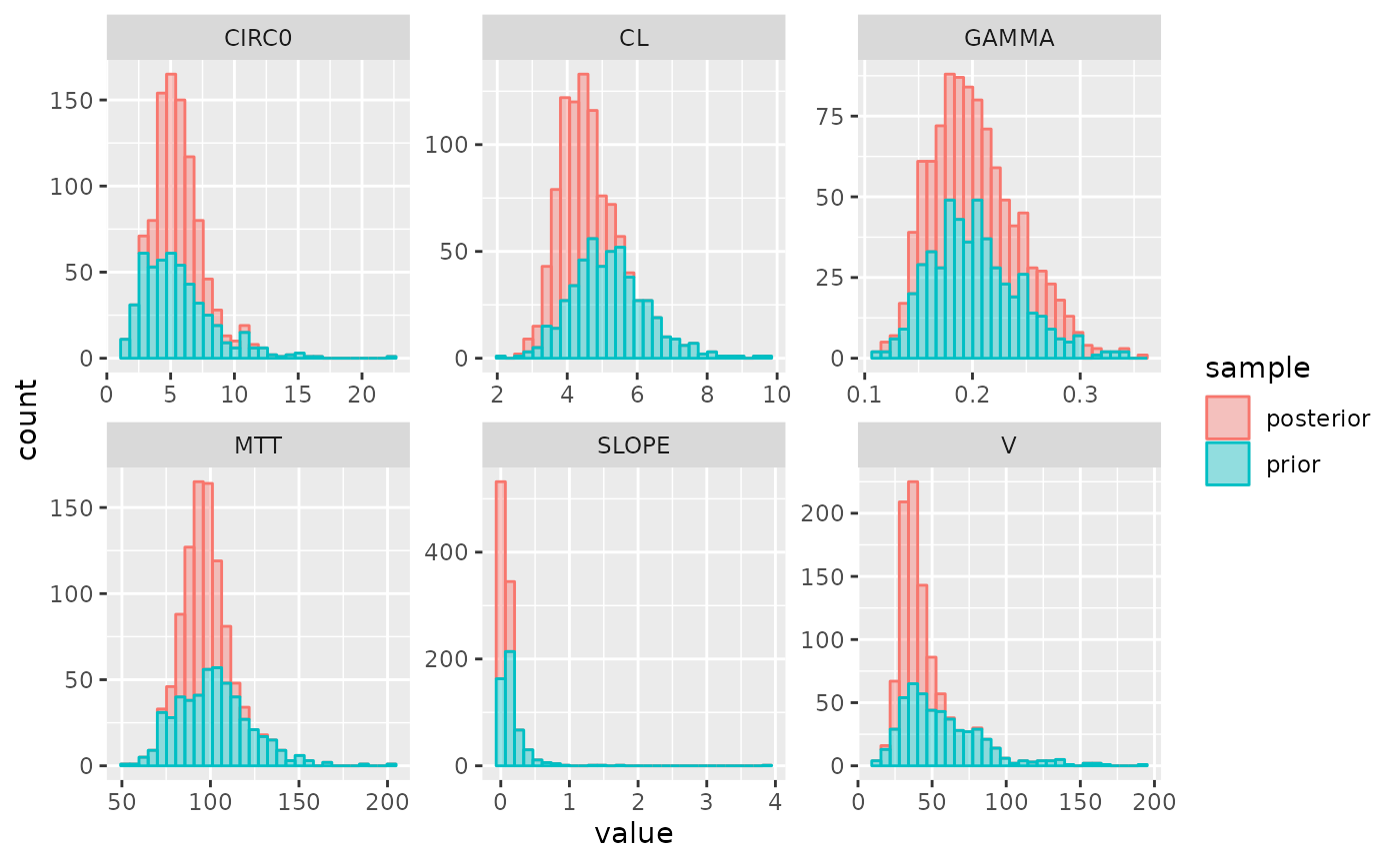
## 6   pd 288.0  2.0  2.0045579 -----|-o--- 0.554  1.2407715  3.024030

Plot parameter distributions:

plot_params(post)