Vancomycin

This examples shows how to implement the vancomycin population PK model published by Thomson et al (JAC 200, http://www.ncbi.nlm.nih.gov/pubmed/19299472), and sample from the posterior for the individual patients after TDM.

We will first create the Stan model and sample from the posterior. Afterwards, we will leverage the PKPDsim model in the pkvancothomson library to simulate the posterior for the dependent variable and create a confidence interval plot.

First, we define the model and parameters:

parameters <- list(
  CL = 2.99, 
  Q = 2.28, 
  V2 = 0.732, 
  V1 = 0.675,
  TH_CRCL = 0.0154,
  TDM_INIT = 0
)
iiv <- list(
  CL = 0.27,
  Q = 0.49, 
  V1 = 0.15, 
  V2 = 1.3
)
ruv <- list(add = 1.6, prop = 0.15)

model <- new_stan_model(
  parameters = parameters,
  parameter_definitions = list(
    "CL" = "CL * (1.0 + TH_CRCL * ((CRCL[j] * 16.6667) - 66.0))",
    "Q"  = "Q",
    "V1" = "V1 * WT[j]",
    "V2" = "V2 * WT[j]",
    "KA" = "0" 
  ),
  fixed = c("TH_CRCL", "TDM_INIT"),
  covariate_definitions = list(
    "CRCL" = "real", # CrCl in L/hr
    "WT" = "real"    # WT in kg
  ),
  solver = "pmx_solve_twocpt",
  scale = "(V1 * mean(WT))",
  verbose = T
)

model_file <- write_stan_model(model)

and compile the model:

mod <- load_model(
  model_file, 
  force = T,
  verbose = T
)

Define the input data and prepare for use in Stan:

regimen <- new_regimen(
  amt = 1500, 
  n = 4, 
  times = c(0, 12, 24, 36), 
  type = 'infusion',
  t_inf = 2
)

covariates <- list(
  WT = new_covariate(value = 70, unit = "kg"),
  CRCL = new_covariate(value = 5, unit = "l/hr")
)

tdm_data <- data.frame(
  t = c(2.5, 11.5), 
  dv = c(40, 14)
)

data <- new_stan_data(
  regimen,
  covariates, 
  tdm_data,
  dose_cmt = 2,
  parameters = parameters,
  fixed = c("TH_CRCL", "TDM_INIT"),
  iiv = iiv,
  ruv = list(
    prop = 0.15,
    add = 1.6
  ),
  ltbs = FALSE
)

Then, we can sample from the posterior using:

post <- get_mcmc_posterior(
  mod = mod,
  data = data
)

## Running MCMC with 1 chain...
## 
## Chain 1 Iteration:   1 / 1000 [  0%]  (Warmup) 
## Chain 1 Iteration:  50 / 1000 [  5%]  (Warmup) 
## Chain 1 Iteration: 100 / 1000 [ 10%]  (Warmup) 
## Chain 1 Iteration: 150 / 1000 [ 15%]  (Warmup) 
## Chain 1 Iteration: 200 / 1000 [ 20%]  (Warmup) 
## Chain 1 Iteration: 250 / 1000 [ 25%]  (Warmup) 
## Chain 1 Iteration: 300 / 1000 [ 30%]  (Warmup) 
## Chain 1 Iteration: 350 / 1000 [ 35%]  (Warmup) 
## Chain 1 Iteration: 400 / 1000 [ 40%]  (Warmup) 
## Chain 1 Iteration: 450 / 1000 [ 45%]  (Warmup) 
## Chain 1 Iteration: 500 / 1000 [ 50%]  (Warmup) 
## Chain 1 Iteration: 501 / 1000 [ 50%]  (Sampling) 
## Chain 1 Iteration: 550 / 1000 [ 55%]  (Sampling) 
## Chain 1 Iteration: 600 / 1000 [ 60%]  (Sampling) 
## Chain 1 Iteration: 650 / 1000 [ 65%]  (Sampling) 
## Chain 1 Iteration: 700 / 1000 [ 70%]  (Sampling) 
## Chain 1 Iteration: 750 / 1000 [ 75%]  (Sampling) 
## Chain 1 Iteration: 800 / 1000 [ 80%]  (Sampling) 
## Chain 1 Iteration: 850 / 1000 [ 85%]  (Sampling) 
## Chain 1 Iteration: 900 / 1000 [ 90%]  (Sampling) 
## Chain 1 Iteration: 950 / 1000 [ 95%]  (Sampling) 
## Chain 1 Iteration: 1000 / 1000 [100%]  (Sampling) 
## Chain 1 finished in 0.3 seconds.

Summary info about the posterior:

post

## Parameters:
##          posterior_mode  mean median    sd    q5   q95  rhat
## CL                2.477 2.508  2.484 0.500 1.730 3.396 0.999
## Q                 1.595 2.015  1.822 0.919 0.949 3.760 0.999
## V2                0.263 1.191  0.467 2.103 0.081 4.274 1.000
## V1                0.567 0.582  0.579 0.063 0.482 0.691 1.003
## TH_CRCL           0.015 0.015  0.015 0.000 0.015 0.015    NA
## TDM_INIT         -0.002 0.000  0.000 0.000 0.000 0.000    NA
## 
## Observed data, posterior:
##   type time dv     mean         loc   pct      pct5    pct95
## 1   pk  2.5 40 30.99324 -----|----o 0.992 26.554420 35.95100
## 2   pk 11.5 14 12.46177 -----|---o- 0.772  9.294978 15.76241

Plot parameter distributions:

plot_params(post)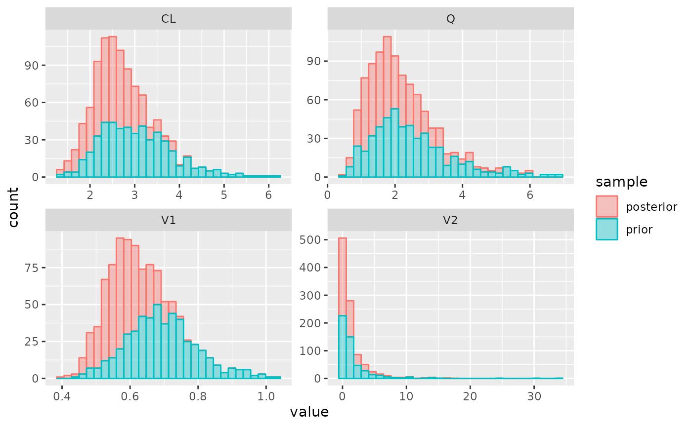

We can now generate the posterior for the dependent value using the PKPDsim model.

First we define an additional required covariates and a mapping between parameters in the PKPDposterior model and the PKPDsim model.

mapping <- list("V1" = "V") # mapping between parameters in the 
covariates$CL_HEMO <- new_covariate(0) # required covariate for PKPDsim model

The PKPDsim model package pkvancothomson that is used in this example can be installed using:

model_from_api(
  system.file("models", "pk_vanco_thomson.json5", package = "PKPDsim"),
  to_package = TRUE,
  install_all = TRUE
)

Then we can simulate the posterior of the dependent variable:

library(pkvancothomson)
pred_post <- sim_from_draws(
  post, 
  model = pkvancothomson::model(),
  map = mapping,
  regimen = regimen,
  covariates = covariates,
  n = 200,
  summarize = TRUE
)
pred_prior <- sim_from_draws(
  post, 
  model = pkvancothomson::model(), 
  map = mapping,
  regimen = regimen,
  covariates = covariates,
  prior = TRUE,
  n = 200,
  summarize = TRUE
)

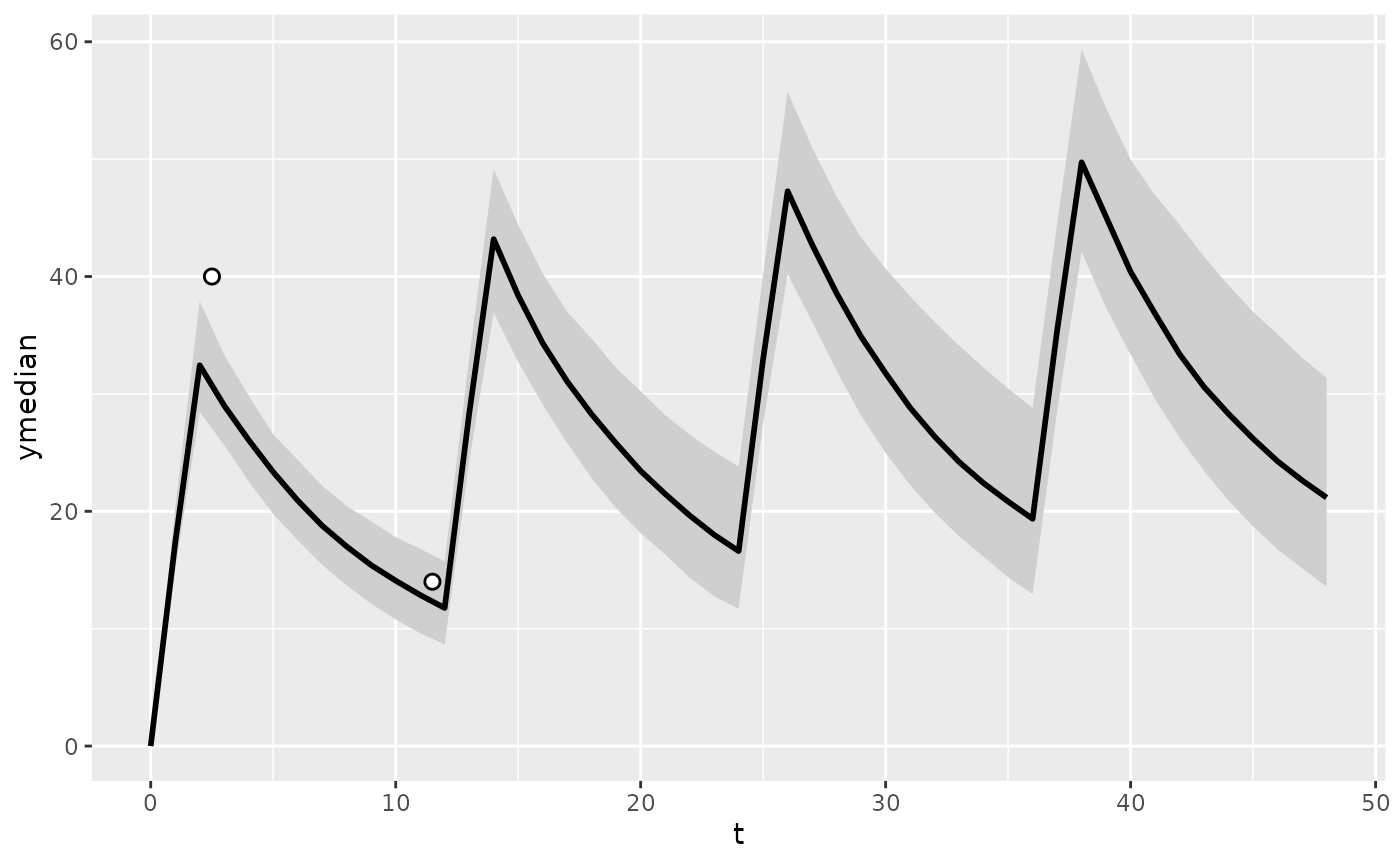
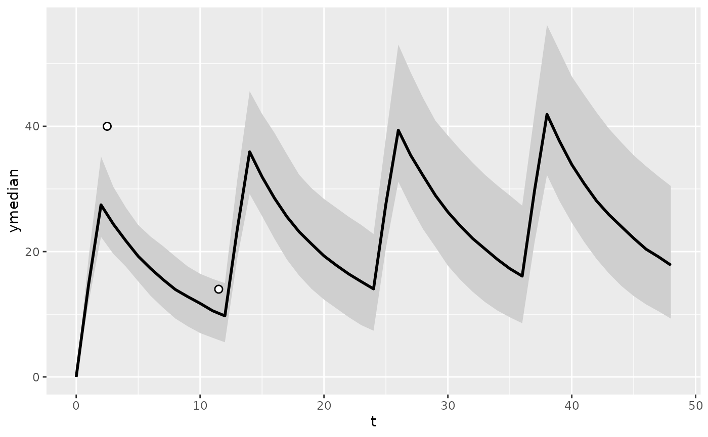
Now we can plot the confidence interval for the posterior and prior predictions using:

plot_predictions(
  pred_prior, 
  obs = tdm_data
)

plot_predictions(
  pred_post, 
  obs = tdm_data
)