Residual error

PKPDsim can simulate residual errors in your observed data, which can be done with the res_var argument to the sim() function. This argument requires a list() with one or more of the following components:

prop: proportional error: \[y = \hat{y} \cdot (1 + \mathcal{N}(0, prop))\]
add: additive error: \[y = \hat{y} + \mathcal{N}(0, add))\]
exp: exponential error: \[y = \hat{y} \cdot e^{\mathcal{N}(0, exp)}\]

These list elements can be combined, e.g. for a combined proportional and additive error model one would write e.g.: res_var = list(prop = 0.1, add = 1), which would give a 10% proportional error plus an additive error of 1 concentration unit.

Below are some examples of the res_var argument

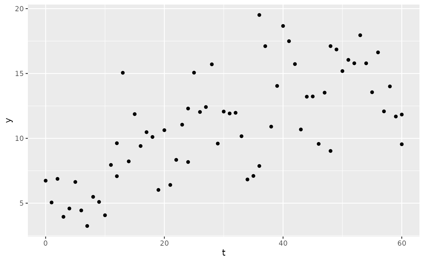
Combined proportional and additive:

mod <- new_ode_model("pk_1cmt_iv")
reg <- new_regimen(
  amt = 1000,
  n = 5,
  interval = 12,
  type = "bolus"
)
sim1 <- sim(
  mod,
  parameters = list(CL = 5, V = 150),
  res_var = list(prop = 0.1, add = 1),
  regimen = reg,
  only_obs=TRUE
)
ggplot(sim1, aes(x = t, y = y)) +
  geom_point()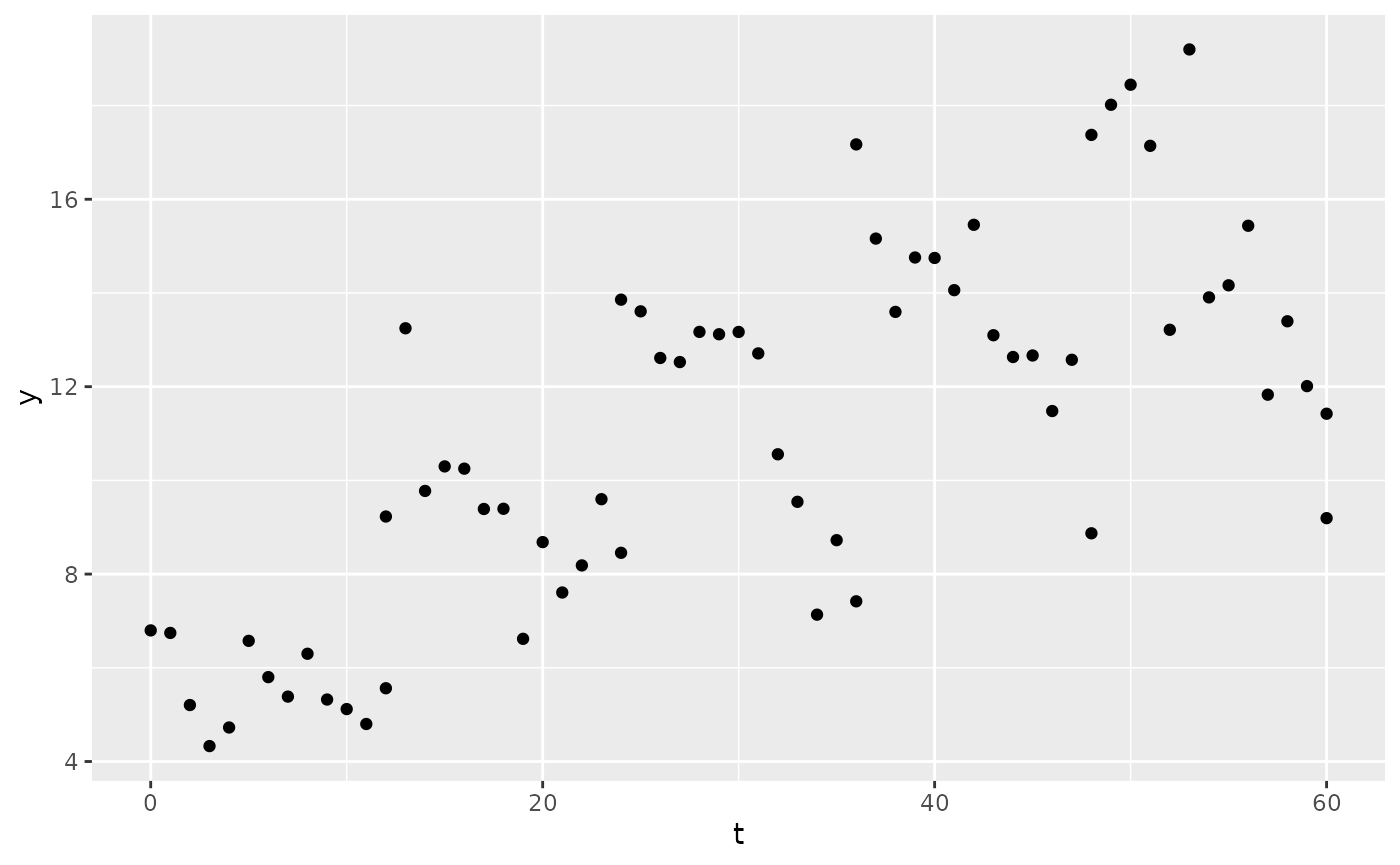

Exponential:

sim2 <- sim(
  mod,
  parameters = list(CL = 5, V = 150),
  res_var = list(exp = 0.1),
  regimen = reg,
  only_obs=TRUE
)

Besides including the residual error at simulation time, there is also the option to include it afterwards. For that, the function add_ruv() is useful.

sim3 <- sim1
sim3$y <- add_ruv(
  x = sim3$y, 
  ruv = list(
    prop = 0.1, 
    add = 1
  )
)
ggplot(sim3, aes(x = t, y = y)) +
  geom_point()