Variability

This can be implemented using the n and omega options. The omega (nomenclature borrowed from NONMEM) should be specified as either a vector defining the lower triangle of the BSV or \(\Omega\) matrix, or as a matrix defining the full \(\Omega\) matrix. An alternative option is to specify the between-subject variability as CV, using the cv_to_omega() function, but this assumes there is no correlation between individual parameters.

The following:

model <- new_ode_model("pk_1cmt_iv")
parameters <- list(CL = 5, V = 50)
regimen <- new_regimen(
  amt = 100,
  n = 3,
  interval = 12,
  type = "infusion",
  t_inf = 2
)

dat <- sim(
  ode = model,
  parameters = parameters,
  regimen = regimen,
  n = 50,
  omega = c(
    0.2, 
    0.05, 0.2
  )
)

will simulate out data for 50 patients, assuming an Omega matrix as defined above. Alternatively, the \(\Omega\) could also have been defined as:

dat <- sim(
  ode = model,
  parameters = parameters,
  regimen = regimen,
  n = 50,
  omega_matrix = matrix(c(
    0.2, 0.05, 
    0.05, 0.2
  ), ncol=2)
)

Or also using the coefficient of variation and without correlation between parameters:

dat <- sim(
  ode = model,
  parameters = parameters,
  regimen = regimen,
  n = 50,
  omega = cv_to_omega(list(
    CL = 0.1, 
    V = 0.1
  ))
)

## No parameter list provided as argument, assumed order for `omega_matrix`: CL, V

Note that using the cv_to_omega function assumes the CV is on the SD-scale and not on the variance scale (and the definition of CV uses the assumption \[1 + \eta \approx 1 * \exp(\eta)\]).

Variability distribution

By default, PKPDsim will assume exponential distribution of all parameters if omega is specified. If normal distribution is desired for all parameters, please use the omega_type argument:

dat <- sim(
  ode = model,
  parameters = parameters,
  regimen = regimen,
  n = 50,
  omega = c(
    0.2, 
    0.05, 0.1
  ),
  omega_type = c("normal", "normal")
)

More flexible variability models

To allow more flexibility in how between-subject variability enters the model, there is an alternative way of specifying variability. This approach is very similar to the way variability is encoded in NONMEM, i.e. variability components (eta’s) are added explicitly in the model code. In PKPDsim this means that eta’s should be treated just like regular parameters, but with 0 mean and normal distribution. 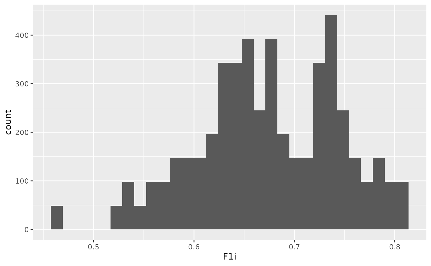See example below for the simulation of bioavailability using the logit-distribution.

mod1 <- new_ode_model(
  code = "
    CLi = CL * exp(eta1)
    Vi = V * exp(eta2)
    F1i =  exp(F1 + eta3) / (1 + exp(F1 + eta3))
    dAdt[1] = -KA * A[1]
    dAdt[2] = KA * A[1] - (CLi/Vi) * A[2]
  ", 
  declare_variables = c("CLi", "Vi", "F1i"),
  obs = list(cmt = 2, scale = "V * exp(eta2)"),
  dose = list(cmt = 1, bioav = "F1i")
)
reg1 <- new_regimen(amt = 100, n = 2, interval = 12, type="oral")
dat <- sim(
  ode = mod1,
  regimen  = reg1,
  parameters = list(
    eta1 = 0,
    eta2 = 0,
    eta3 = 0,
    CL = 5,
    V = 50,
    KA = .5,
    F1 = 0.8
  ),
  t_obs = c(0:48),
  omega = c(
    0.1, 
    0.05, 0.1, 
    0,    0,   0.1
  ),
  n = 100,
  omega_type = c("normal", "normal", "normal"),
  output_include = list("parameters" = TRUE, variables = TRUE),
  only_obs = TRUE
)

library(ggplot2)
ggplot(dat, aes(x = t, y = y, group = id)) + geom_line()

ggplot(dat, aes(x = F1i)) + geom_histogram()

## `stat_bin()` using `bins = 30`. Pick better value with `binwidth`.