PKPD model

Below is an example of a simple indirect-response model. With PK-PD models, the initial state of the PD system often depends on specific model parts. We can define the state of the ODE system statically using the A_init= argument, but this will not take any parameters into account. However, we can also define initial states dynamically using the state_init argument, which allow you to specify the state of each compartment using code.

library("PKPDsim")
library("ggplot2")

p_pkpd <- list(
  CL = 5,
  V  = 50,
  KIN = .02,
  KOUT=.5,
  EFF = 0.2
)

r1 <- new_regimen(
  amt = 100,
  interval = 12,
  n = 5
)

pkpd <- new_ode_model(
  code = "
    dAdt[1] = -(CL/V) * A[1];
    conc = A[1]/V;
    dAdt[2] = KIN * 1/(1+EFF*conc) - KOUT*A[2];
  ",
  state_init = "A[2] = KIN/KOUT;"
)

dat <- sim(
  ode = pkpd,
  n_ind = 25,
  omega = cv_to_omega(
    par_cv = list(CL = 0.1, V = 0.1, KIN = .05, KOUT = 0.1),
    p_pkpd
  ),
  parameters = p_pkpd,
  regimen = r1,
  verbose = FALSE
)

ggplot(dat, aes(x = t, y = y, colour = factor(id))) +
  geom_line() +
  scale_colour_discrete(guide = "none") +
  facet_wrap(~comp, scales = "free")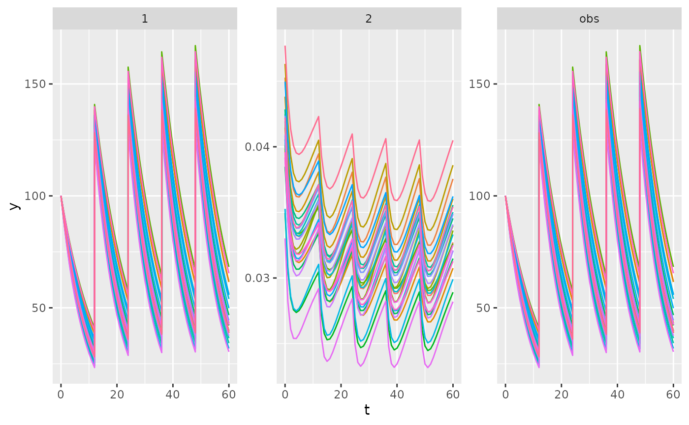

Combine PK and PD models

As shown above, a PK-PD model can be written as a single set of differential equations. However, we often develop PK and PD models separately and e.g. want to plug various PK models into existing PD models. In PKPDsim you can two or more model parts separately in a list to the code argument:

pkpd <- new_ode_model(
  code = list(
    pk = "dAdt[1] = -(CL/V) * A[1]; conc = A[1]/V; ",
    pd = " dAdt[1] = KIN * 1/(1+EFF*conc) - KOUT*A[1]; "
  ),
  state_init = list(pd = "A[1] = KIN/KOUT;")
)

The above two systems of ODEs will then be combined into a single one.